https://pyimagesearch.com/2022/02/28/multi-column-table-ocr/
Multi-Column Table OCR
by Adrian Rosebrock on February 28, 2022 Click here to download the source code to this post

- Discover a technique for associating rows and columns together
- Learn how to detect tables of text/data in an image
- Extract the detected table from an image
- OCR the text in the table
- Apply hierarchical agglomerative clustering (HAC) to associate rows and columns
- Build a Pandas
DataFramefrom the OCR’d data
This tutorial is the first in a 4-part series on OCR with Python:
- Multi-Column Table OCR (this tutorial)
- OpenCV Fast Fourier Transform (FFT) for Blur Detection in Images and Video Streams
- OCR’ing Video Streams
- Improving Text Detection Speed with OpenCV and GPUs
To learn how to OCR multi-column tables, just keep reading.
Looking for the source code to this post?
JUMP RIGHT TO THE DOWNLOADS SECTIONMulti-Column Table OCR
Perhaps one of the more challenging applications of optical character recognition (OCR) is how to successfully OCR multi-column data (e.g., spreadsheets, tables, etc.).
On the surface, OCR’ing tables seems like it should be an easier problem, right? However, given that the document has a guaranteed structure, shouldn’t we leverage this a priori knowledge and then OCR each column in the table?
In most cases, yes, that would be the case. But unfortunately, we have a few problems to address:
- Tesseract isn’t very good at multi-column OCR, especially if your image is noisy.
- You may need first to detect the table in the image before you can OCR it.
- Your OCR engine (Tesseract, cloud-based, etc.) may correctly OCR the text but be unable to associate the text into columns/rows.
So, while OCR’ing multi-column data may appear to be an easy task, it’s far harder since we may need to be responsible for associating text into columns and rows — and as you’ll see, that is indeed the most complex part of our implementation.
The good news is that while OCR’ing multi-column data is certainly more demanding than other OCR tasks, it’s not a “hard problem,” provided you bring the right algorithms and techniques to the project.
In this tutorial, you’ll learn some tips and tricks to OCR multi-column data, and most importantly, associate rows/columns of text together.
OCR’ing Multi-Column Data
In the first part of this tutorial, we’ll discuss our multi-column OCR algorithm’s basic process. This is the exact algorithm to OCR multi-column data. It serves as a great starting point, and we recommend using it whenever you need to OCR a table.
From there, we’ll review the directory structure for our project. We’ll also install any additional required Python packages for the tutorial.
With our development environment fully configured, we can move on to our implementation. We’ll spend most of the lesson here, covering our multi-column OCR algorithm’s details and inner workings.
We’ll wrap up the lesson by applying our Python implementation to:
- Detect a table of text in an image
- Extract the table
- OCR the table
- Build a Pandas
DataFramefrom the table to process it, query it, etc.
Our Multi-Column OCR Algorithm
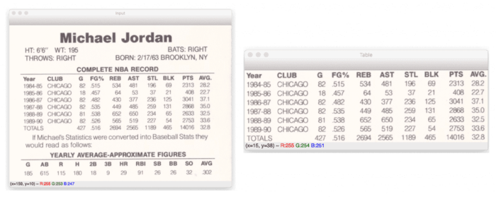
Our multi-column OCR algorithm is a multi-step process. To start, we need to accept an input image containing a table, spreadsheet, etc. (Figure 1, left). Given this image, we then need to extract the table itself (right).
Once we have the table, we can apply OCR and text localization to generate the (x, y)-coordinates for the text bounding boxes. It’s paramount that we obtain these bounding box coordinates.
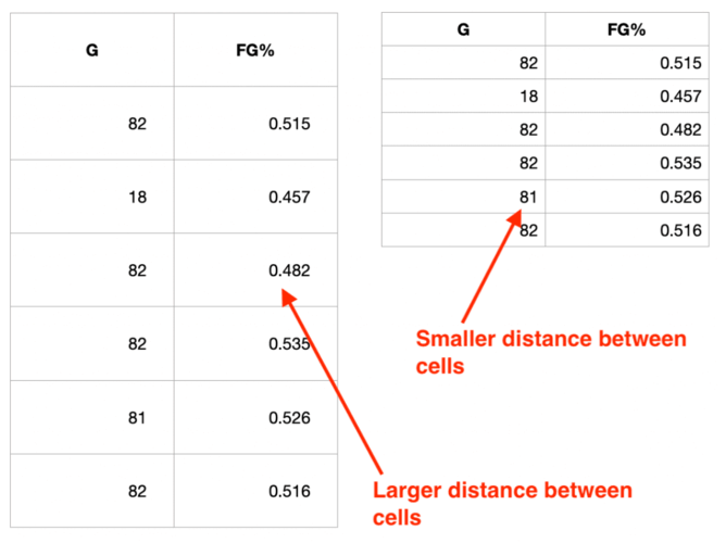
To associate columns of text together, we need to group pieces of text based on their starting x-coordinate.
Why starting x-coordinate? Well, keep in mind the structure of a table, spreadsheet, etc. Each column’s text will have near-identical starting x-coordinates because they belong to the same column (take a second now to convince yourself that the statement is true).
We can thus exploit that knowledge and then cluster groups of text together with near-identical x-coordinates.
But the question remains, how do we do the actual grouping?
The answer is to use a special clustering algorithm called hierarchical agglomerative clustering (HAC). If you’ve ever taken a data science, machine learning, or text mining class before, then you’ve likely encountered HAC previously.
A full review of the HAC algorithm is outside the scope of this tutorial. Still, the general idea is that we take a “bottom-up” approach, starting with our initial data points (i.e., the x-coordinates of the text bounding boxes) as individual clusters, each containing only one observation.
We then compute the distance between the coordinates and start grouping observations with a distance < T, where T is a pre-defined threshold.
At each iteration of HAC, we choose the two clusters with the smallest distance and merge them, again, provided that the distance threshold requirement is met.
We continue clustering until no other clusters can be formed, typically because no two clusters fall within our threshold requirement.
In the context of multi-column OCR, applying HAC to the x-coordinate value results in clusters that have identical or near-identical x-coordinates. And since we assume that text belonging to the same column will have similar/near-identical x-coordinates, we can associate columns together.
While this technique to multi-column OCR may seem complicated, it’s straightforward, especially since we’ll be able to utilize the AgglomerativeClustering implementation in the scikit-learn library.
That said, implementing agglomerative clustering by hand is a good exercise if you are interested in learning more about machine learning and data science techniques. I’ve had to implement HAC 3-4 times before in my career, predominately when I was in college.
If you want to learn more about HAC, I recommend the scikit-learn documentation and the excellent article by Cory Maklin.
For a more theoretical and mathematically motivated treatment of agglomerative clustering, including clustering algorithms in general, I highly recommend Data Mining: Practical Machine Learning Tools and Techniques by Witten et al. (2011).
Configuring Your Development Environment
To follow this guide, you need to have the OpenCV library installed on your system.
Luckily, OpenCV is pip-installable:
→ Launch Jupyter Notebook on Google ColabIf you need help configuring your development environment for OpenCV, we highly recommend that you read our pip install OpenCV guide — it will have you up and running in a matter of minutes.
Having Problems Configuring Your Development Environment?
All that said, are you:
- Short on time?
- Learning on your employer’s administratively locked system?
- Wanting to skip the hassle of fighting with the command line, package managers, and virtual environments?
- Ready to run the code right now on your Windows, macOS, or Linux system?
Then join PyImageSearch University today!
Gain access to Jupyter Notebooks for this tutorial and other PyImageSearch guides that are pre-configured to run on Google Colab’s ecosystem right in your web browser! No installation required.
And best of all, these Jupyter Notebooks will run on Windows, macOS, and Linux!
Project Structure
Start by accessing the “Downloads” section of this tutorial to retrieve the source code and example images.
Next, let’s review our project directory structure:
→ Launch Jupyter Notebook on Google ColabAs you can see, our project directory structure is quite simple — but don’t let the simplicity fool you!
Our
For reference, our example image is a scan of the Michael Jordan baseball card (Figure 3), when he took a year off from basketball to play baseball after his father died.
Our Python script can OCR the table, parse out his stats, and then output them as OCR’d text as a CSV file (
Installing Required Packages
Our Python script will display a nicely formatted table of OCR’d text to our terminal. Still, we need to utilize the
Python package to generate this formatted table.You can install
If you are using Python virtual environments, don’t forget to use the
Again, the
Implementing Multi-Column OCR
We are now ready to implement multi-column OCR! Open the
# import the necessary packages
from sklearn.cluster import AgglomerativeClustering
from pytesseract import Output
from tabulate import tabulate
import pandas as pd
import numpy as np
import pytesseract
import argparse
import imutils
import cv2
We start by importing our required Python packages. We have several packages we haven’t (or at the very least, not often) worked with before, so let’s review the important ones.
First, we have our
The
We then have the
The rest of the imports should look familiar to you, as we have used each of them many times throughout our lessons.
Let’s move on to our command line arguments:
→ Launch Jupyter Notebook on Google Colab# construct the argument parser and parse the arguments
ap = argparse.ArgumentParser()
ap.add_argument("-i", "--image", required=True,
help="path to input image to be OCR'd")
ap.add_argument("-o", "--output", required=True,
help="path to output CSV file")
ap.add_argument("-c", "--min-conf", type=int, default=0,
help="minimum confidence value to filter weak text detection")
ap.add_argument("-d", "--dist-thresh", type=float, default=25.0,
help="distance threshold cutoff for clustering")
ap.add_argument("-s", "--min-size", type=int, default=2,
help="minimum cluster size (i.e., # of entries in column)")
args = vars(ap.parse_args())As you can see, we have several command line arguments. Let’s discuss each of them:
-
--image: The path to the input image containing the table, spreadsheet, etc., that we want to detect and OCR
-
--output: Path to the output CSV file that will contain the column data we extracted
-
--min-conf: Used to filter out weak text detections
-
--dist-thresh: Distance threshold cutoff (in pixels) for when applying HAC; you may need to tune this value for your images and datasets
-
--min-size: Minimum number of data points in a cluster for it to be considered a column
The most important command line arguments here are
When applying HAC, we need to use a distance threshold cutoff. If you allow clustering to continue indefinitely, HAC will continue to cluster at each iteration until you end up, trivially, with one cluster that contains all data points.
Instead, you apply a distance threshold to stop the clustering process when no two clusters have a distance less than the threshold.
For your purposes, you’ll need to examine the image data with which you are working. If your tabular data have large amounts of whitespace between each row, then you’ll likely need to increase the
Otherwise, if there is less whitespace between each row, the
Setting your
The
However, there will always be outliers, pieces of text that are far outside the table, or just noise in the image. If Tesseract detects this text, then HAC will try to cluster it. But is there a way to prevent these clusters from being reported in our results?
A simple way is to check the number of text data points inside a given cluster after HAC is complete.
In this case, we set
With our command line arguments taken care of, let’s start our image processing pipeline:
→ Launch Jupyter Notebook on Google Colab# set a seed for our random number generator
np.random.seed(42)
# load the input image and convert it to grayscale
image = cv2.imread(args["image"])
gray = cv2.cvtColor(image, cv2.COLOR_BGR2GRAY)Line 27 sets the seed of our pseudorandom number generator. We do this to generate colors for each column of text we detect (useful for visualization purposes).
We then load our input
Our next code block detects large blocks of text in our
# initialize a rectangular kernel that is ~5x wider than it is tall,
# then smooth the image using a 3x3 Gaussian blur and then apply a
# blackhat morphological operator to find dark regions on a light
# background
kernel = cv2.getStructuringElement(cv2.MORPH_RECT, (51, 11))
gray = cv2.GaussianBlur(gray, (3, 3), 0)
blackhat = cv2.morphologyEx(gray, cv2.MORPH_BLACKHAT, kernel)

# compute the Scharr gradient of the blackhat image and scale the
# result into the range [0, 255]
grad = cv2.Sobel(blackhat, ddepth=cv2.CV_32F, dx=1, dy=0, ksize=-1)
grad = np.absolute(grad)
(minVal, maxVal) = (np.min(grad), np.max(grad))
grad = (grad - minVal) / (maxVal - minVal)
grad = (grad * 255).astype("uint8")

# apply a closing operation using the rectangular kernel to close
# gaps in between characters, apply Otsu's thresholding method, and
# finally a dilation operation to enlarge foreground regions
grad = cv2.morphologyEx(grad, cv2.MORPH_CLOSE, kernel)
thresh = cv2.threshold(grad, 0, 255,
cv2.THRESH_BINARY | cv2.THRESH_OTSU)[1]
thresh = cv2.dilate(thresh, None, iterations=3)
cv2.imshow("Thresh", thresh)
First, we construct a large rectangular kernel that is
The next step is to compute the gradient magnitude representation of the blackhat image and scale the output image back to the range
We can now apply a closing operation (Line 52). We use our large rectangular
We finish the pipeline by thresholding the image and applying a series of dilations to enlarge foreground regions.
Figure 5 displays the output of this pre-processing pipeline. On the left, we have our original input image. This image is the back of a Michael Jordan baseball card (when he left the NBA for a year to play baseball). Since they didn’t have any baseball stats for Jordan, they included his basketball stats on the back of the card, despite being a baseball card (weird, I know, which is also why his baseball cards are collector’s items).
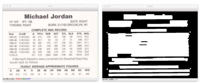
Our goal is to OCR his “Complete NBA Record” table. And if you look at Figure 5 (right), you can see that the table is visible as one big rectangular-like blob.
Our next code block handles detecting and extracting this table:
→ Launch Jupyter Notebook on Google Colab# find contours in the thresholded image and grab the largest one,
# which we will assume is the stats table
cnts = cv2.findContours(thresh.copy(), cv2.RETR_EXTERNAL,
cv2.CHAIN_APPROX_SIMPLE)
cnts = imutils.grab_contours(cnts)
tableCnt = max(cnts, key=cv2.contourArea)
# compute the bounding box coordinates of the stats table and extract
# the table from the input image
(x, y, w, h) = cv2.boundingRect(tableCnt)
table = image[y:y + h, x:x + w]
# show the original input image and extracted table to our screen
cv2.imshow("Input", image)
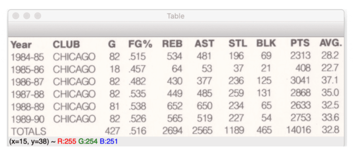
cv2.imshow("Table", table)First, we detect all contours in our thresholded image (Lines 60-62). We then find the single largest contour based on the area of the contour (Line 63).
We’re assuming that the single largest contour is our table, and as we can verify from Figure 5 (right), that is indeed the case. However, you may need to update the contour processing to find the table using other methods for your projects. The method covered here is certainly not a one-size-fits-all solution.
Given the contour corresponding to the table,
The extracted
Now that we have our statistics
# set the PSM mode to detect sparse text, and then localize text in
# the table
options = "--psm 6"
results = pytesseract.image_to_data(
cv2.cvtColor(table, cv2.COLOR_BGR2RGB),
config=options,
output_type=Output.DICT)

# initialize a list to store the (x, y)-coordinates of the detected
# text along with the OCR'd text itself
coords = []
ocrText = []
Lines 76-80 use Tesseract to compute bounding box locations for each piece of text in the
Additionally, notice how we are using
Most tables of data are going to be uniform. They will leverage near-identical font and font sizes.
If
After applying OCR text detection, we initialize two lists:
Let’s move on to looping over each of our text detections:
→ Launch Jupyter Notebook on Google Colab# loop over each of the individual text localizations
for i in range(0, len(results["text"])):
# extract the bounding box coordinates of the text region from
# the current result
x = results["left"][i]
y = results["top"][i]
w = results["width"][i]
h = results["height"][i]
# extract the OCR text itself along with the confidence of the
# text localization
text = results["text"][i]
conf = int(results["conf"][i])
# filter out weak confidence text localizations
if conf > args["min_conf"]:
# update our text bounding box coordinates and OCR'd text,
# respectively
coords.append((x, y, w, h))
ocrText.append(text)Lines 91-94 extract the bounding box coordinates from the detected text region, while Lines 98 and 99 extract the OCR’d text itself, along with the confidence of the text detection.
Line 102 filters out weak text detections. If the
We can now move on to the clustering phase of the project:
→ Launch Jupyter Notebook on Google Colab# extract all x-coordinates from the text bounding boxes, setting the
# y-coordinate value to zero
xCoords = [(c[0], 0) for c in coords]
# apply hierarchical agglomerative clustering to the coordinates
clustering = AgglomerativeClustering(
n_clusters=None,
affinity="manhattan",
linkage="complete",
distance_threshold=args["dist_thresh"])
clustering.fit(xCoords)
# initialize our list of sorted clusters
sortedClusters = []Line 110 extracts all x-coordinates from the text bounding boxes. Notice how we are forming a proper (x, y)-coordinate tuple here but setting y = 0 for each entry. Why is y set to 0 ?
The answer is two-fold:
- First, to apply HAC, we need a set of input vectors (also called “feature vectors”). Our input vectors must be at least 2-D, so we add a trivial dimension containing a value of
0.
- Secondly, we aren’t interested in the y-coordinate value. We only want to cluster on the x-coordinate positions. Pieces of text with similar x-coordinates are likely to be part of a column in a table.
From there, Lines 113-118 apply hierarchical agglomerative clustering. We set
Also, note that we are using the Manhattan distance function here. Why not some other distance function (e.g., Euclidean)?
While you can (and should) experiment with our distance metrics, Manhattan tends to be an appropriate choice here. We want to be very stringent on our requirement that x-coordinates lie close together. But again, I suggest you experiment with other distance methods.
For more details on scikit-learn’s
Now that our clustering is complete, let’s loop over each of the unique clusters:
→ Launch Jupyter Notebook on Google Colab# loop over all clusters
for l in np.unique(clustering.labels_):
# extract the indexes for the coordinates belonging to the
# current cluster
idxs = np.where(clustering.labels_ == l)[0]
# verify that the cluster is sufficiently large
if len(idxs) > args["min_size"]:
# compute the average x-coordinate value of the cluster and
# update our clusters list with the current label and the
# average x-coordinate
avg = np.average([coords[i][0] for i in idxs])
sortedClusters.append((l, avg))
# sort the clusters by their average x-coordinate and initialize our
# data frame
sortedClusters.sort(key=lambda x: x[1])
df = pd.DataFrame()Line 130 then verifies that the current cluster has more than --min-size items inside of it.
We then compute the average of the x-coordinates inside the cluster and update our sortedClusters
list with a 2-tuple containing the current label, l , along with the average x-coordinate value.Line 139 sorts our sortedClusters list based on our average x-coordinate. We perform this sorting operation such that our clusters are sorted left-to-right across the page.
Finally, we initialize an empty DataFrame to store our multi-column OCR results.
Let’s now loop over our sorted clusters:
→ Launch Jupyter Notebook on Google Colab# loop over the clusters again, this time in sorted order
for (l, _) in sortedClusters:
# extract the indexes for the coordinates belonging to the
# current cluster
idxs = np.where(clustering.labels_ == l)[0]
# extract the y-coordinates from the elements in the current
# cluster, then sort them from top-to-bottom
yCoords = [coords[i][1] for i in idxs]
sortedIdxs = idxs[np.argsort(yCoords)]
# generate a random color for the cluster
color = np.random.randint(0, 255, size=(3,), dtype="int")
color = [int(c) for c in color]Line 143 loops over the labels in our sortedClusters list. We then find the indexes (idxs) of all data points belonging to the current cluster label, l .
Using the indexes, we extract the y-coordinates from all pieces of text in the cluster and sort them from top-to-bottom (Lines 150 and 151).
We also initialize a random color for the current column (so we can visualize which pieces of text belong to which column).
Let’s loop over each of the pieces of text in the column now:
→ Launch Jupyter Notebook on Google ColabMulti-Column Table OCR
# loop over the sorted indexes
for i in sortedIdxs:
# extract the text bounding box coordinates and draw the
# bounding box surrounding the current element
(x, y, w, h) = coords[i]
cv2.rectangle(table, (x, y), (x + w, y + h), color, 2)
# extract the OCR'd text for the current column, then construct
# a data frame for the data where the first entry in our column
# serves as the header
cols = [ocrText[i].strip() for i in sortedIdxs]
currentDF = pd.DataFrame({cols[0]: cols[1:]})
# concatenate *original* data frame with the *current* data
# frame (we do this to handle columns that may have a varying
# number of rows)
df = pd.concat([df, currentDF], axis=1)For each
We then grab all pieces of
Now that we’ve extracted the current column, we create a separate
Finally, we concatenate our original data frame,
At this point, our table OCR process is complete, and we just need to save the table to disk:
→ Launch Jupyter Notebook on Google Colab → Launch Jupyter Notebook on Google ColabIf some columns have more entries than others, then the empty entries will be filled with a “Not a Number” (
Line 178 displays a nicely formatted table to our terminal, demonstrating that we’ve OCR’d the multi-column data successfully.
We then save our data frame to disk as a CSV file on Line 182.
Finally, we display our output image to our screen on Line 185.
Multi-Column OCR Results
We are now ready to see our multi-column OCR script in action!
Open a terminal and execute the following command:
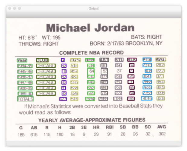
→ Launch Jupyter Notebook on Google Colab → Launch Jupyter Notebook on Google ColabFigure 7 (top) displays the extracted table. We then apply hierarchical agglomerative clustering (HAC) to OCR the table, resulting in the bottom figure.
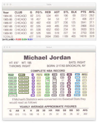
Notice how we have color-coded the columns of text. Text with the same bounding box color belongs to the same column, demonstrating that our HAC method successfully associated columns of text together.
A text version of our OCR’d table can be seen in the terminal output above. Our OCR results are very accurate for the most part, but there are a few notable issues to call out.
To start, the field goal percentage (
The same issue can be found in the average points per game (
This one is slightly harder to resolve, though. If we were to cast to a
- Check the length of the string
- If the string has four characters, then the decimal point has already been added, so no further work is required
- Otherwise, the string has three characters, so insert a decimal point between the second and third characters
Any time you can leverage any a priori knowledge regarding the OCR task at hand, the far easier time you’ll have. In this case, our domain knowledge tells us which columns should have decimal points, so we can leverage text post-processing heuristics to improve our OCR results further, even when Tesseract performs less than optimally.
The most significant issues with our OCR results can be found in the
Since this tutorial focuses specifically on OCR’ing multi-column data, and most importantly, the algorithm powering it, we’re not going to spend a ton of time focusing on improvements to Tesseract options and configurations here.
After our Python script has been executed, we have an output
→ Launch Jupyter Notebook on Google Colab → Launch Jupyter Notebook on Google Colab
As you can see, our OCR’d table has been written to disk as a CSV file. You can take this CSV file and process it using data mining techniques.
What's next? I recommend PyImageSearch University.


35+ total classes • 39h 44m video • Last updated: April 2022
★★★★★ 4.84 (128 Ratings) • 13,800+ Students Enrolled
I strongly believe that if you had the right teacher you could master computer vision and deep learning.
Do you think learning computer vision and deep learning has to be time-consuming, overwhelming, and complicated? Or has to involve complex mathematics and equations? Or requires a degree in computer science?
That’s not the case.
All you need to master computer vision and deep learning is for someone to explain things to you in simple, intuitive terms. And that’s exactly what I do. My mission is to change education and how complex Artificial Intelligence topics are taught.
If you're serious about learning computer vision, your next stop should be PyImageSearch University, the most comprehensive computer vision, deep learning, and OpenCV course online today. Here you’ll learn how to successfully and confidently apply computer vision to your work, research, and projects. Join me in computer vision mastery.
Inside PyImageSearch University you'll find:
- ✓ 35+ courses on essential computer vision, deep learning, and OpenCV topics
- ✓ 35+ Certificates of Completion
- ✓ 39+ hours of on-demand video
- ✓ Brand new courses released regularly, ensuring you can keep up with state-of-the-art techniques
- ✓ Pre-configured Jupyter Notebooks in Google Colab
- ✓ Run all code examples in your web browser — works on Windows, macOS, and Linux (no dev environment configuration required!)
- ✓ Access to centralized code repos for all 450+ tutorials on PyImageSearch
- ✓ Easy one-click downloads for code, datasets, pre-trained models, etc.
- ✓ Access on mobile, laptop, desktop, etc.
Summary
In this tutorial, you learned how to OCR multi-column data using the Tesseract OCR engine and hierarchical agglomerative clustering (HAC).
Our multi-column OCR algorithm works by:
- Detecting tables of text in an input image using gradients and morphological operations
- Extracting the detected table
- Using Tesseract (or equivalent) to localize text in the table and extract the bounding box (x, y)-coordinates of the text in the table
- Applying HAC to cluster on the x-coordinate of the table with a maximum distance threshold cutoff
Essentially what we are doing here is grouping text localizations with x-coordinates that are either identical or very close to each other.
Why does this method work?
Well, consider the structure of a spreadsheet, table, or any other document that has multiple columns. In that case, the data in each column will have near identical starting x-coordinates because they belong to the same column. We can thus exploit that knowledge and then cluster groups of text together with near-identical x-coordinates.
While this method is simplistic, it works quite well in practice.
Citation Information
Rosebrock, A. “Multi-Column Table OCR,” PyImageSearch, 2022, https://pyimg.co/h18s2
Want free GPU credits to train models?
- We used Jarvislabs.ai, a GPU cloud, for all the experiments.
- We are proud to offer PyImageSearch University students $20 worth of Jarvislabs.ai GPU cloud credits. Join PyImageSearch University and claim your $20 credit here.
In Deep Learning, we need to train Neural Networks. These Neural Networks can be trained on a CPU but take a lot of time. Moreover, sometimes these networks do not even fit (run) on a CPU.
To overcome this problem, we use GPUs. The problem is these GPUs are expensive and become outdated quickly.
GPUs are great because they take your Neural Network and train it quickly. The problem is that GPUs are expensive, so you don’t want to buy one and use it only occasionally. Cloud GPUs let you use a GPU and only pay for the time you are running the GPU. It’s a brilliant idea that saves you money.
JarvisLabs provides the best-in-class GPUs, and PyImageSearch University students get between 10-50 hours on a world-class GPU (time depends on the specific GPU you select).
This gives you a chance to test-drive a monstrously powerful GPU on any of our tutorials in a jiffy. So join PyImageSearch University today and try it for yourself.
To download the source code to this post (and be notified when future tutorials are published here on PyImageSearch), simply enter your email address in the form below!
